This is a continuation of the
Process Intensifier - Optimization with CFD: Part 1 paper.
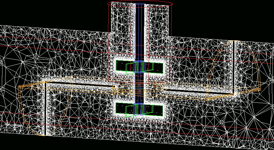
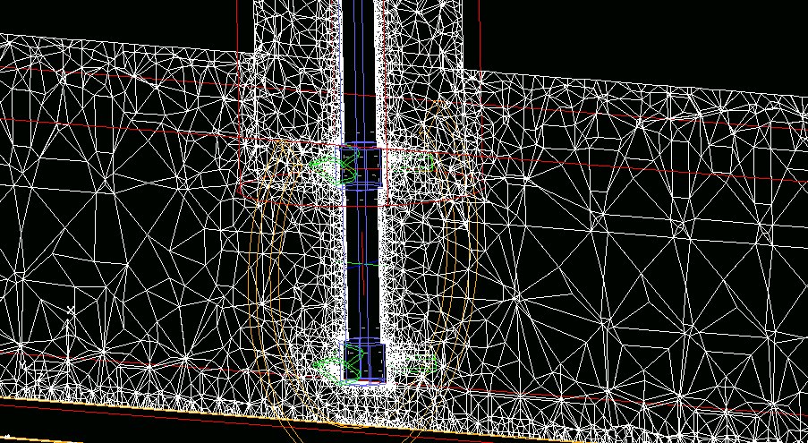
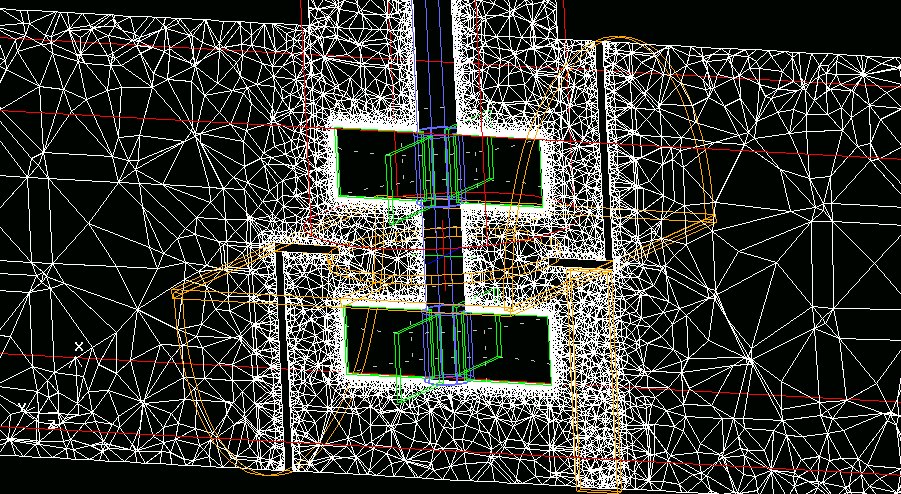
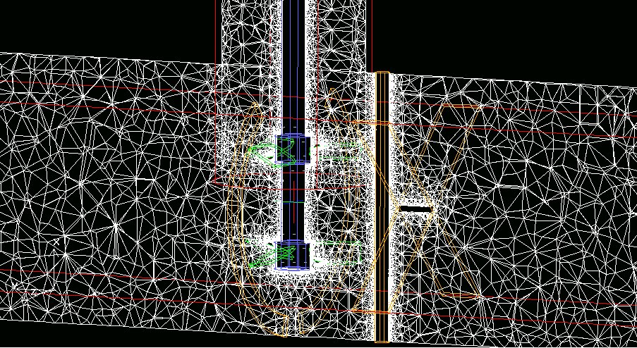
CFD is a great tool to determine velocity profiles, flow patterns, dead zones, and possible short-circuiting. The ACUSOLVE mesh generator does not generate evenly spaced cells, but decides where it needs better resolution and where it does not. Therefore ACUSOLVE generates a finer grid of tetrahedra near solid surfaces, moving and stationary, than in the bulk of the fluid (see Figure 9). This automatic descretization can be also overruled in order to make an even finer grid in desired areas (such as areas of flow detachment and reattachment).
| CFD Mesh
|
Radial Process Intensifier
|
Axial
Process Intensifier
|
| Lightnin |
 |
 |
| |
Z-plate, impellers, shaft
1.2 million tetras |
Impellers, shaft, injection tube, baffles
1.1 million tetras |
| Hayward Gordon |
 |
 |
| |
Z-plate, impellers, shaft
956,000 tetras |
Impellers, shaft, baffles
1.4 million tetras |
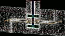
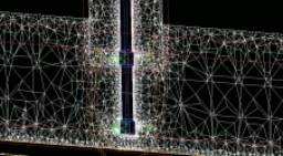
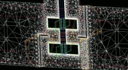
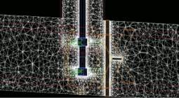
| Figure
10: Meshing of the active mixing zone. The whiter areas are areas
having a finer mesh. Click on any picture to get a larger
view. See the blades, plates, baffles, etc. |
It may look (Figure 10) as though there are no impeller blades for the Axial
Process Intensifier, but that is because the impellers have 3 blades and none of
them intersect the central vertical plane. Two of the four blades of the radial
impellers intersect this plane.
Although it may appear that the Radial Process Intensifiers have about the
same mesh density as the Axials, there are fewer "small" tetrahedra in
the axial flow models because there is less total internal surface area. In the
Radial Process intensifiers, there are four blades instead of 3 and there is the
complete Z-plate that needs to be meshed, which has a much larger surface area
than the horseshoe baffle (isn't very visible in this vertical plane because it
is perpendicular to it). The grid density over the radial impeller blade
thickness is not very high, so we used the Spalart-Allmaras turbulence Model to
assist in the boundary layer and other general turbulence effects. The
rotational reference frame around each impeller is very tight. It is about 6 mm
spaced from the rotating surfaces.
From a general principle perspective, as the mesh becomes more dense, the
accuracy of the solution improves, along with the necessary increase in
computing time. After a brief mesh resolution sensitivity study using meshes
that were more coarse, we found that with models on the order of 0.8 Million to
1.4 million tetrahedra depending on the subject, we could achieve sufficient
accuracy relative to the body of experimental data relative to the torque,
power, and power numbers. These models tended to converge in the range of 20 to
30 nonlinear iterations, to a normalized residual tolerance of less than 1.0
E-3.
Further, for the models in that range, we found that the solutions could be
run on a 1.8 GHz laptop computer with 512 MB of memory in roughly 2 hours.
However, we also did most of the runs on a parallel configuration of two 2.0 GHz
with 2.0 GB memory each, and the solutions required only about 30 minutes each.
This phenomenal computing speed enabled the completion of the computational
aspects of this work in a very reasonable time, which was faster than the time
required to have done all of the experiments.
Continue with Velocity Profiles
or
Go back to Results
or
Go back to the Title Page
|