This is a continuation of the
Process Intensifier - Optimization with CFD: Part 1 paper.
This is a continuation of the Process
Intensifier - Optimization with CFD: Part 1 paper.
The sequences of velocity images are all 3-D vectors, but shown here mainly
directly normal to each plane so they basically appear as 2-D vectors. A 3-D
vector that is exactly normal to the viewing plane would not appear as a point
but rather as a plus sign that is proportional in size to the vector magnitude.
The reason for this is that the 3-D vector has the arrow made up of orthogonal
V's. 3-D vectors provide primarily two functions here. The first is that they
can be viewed from any orientation, so that out of plane motion can be seen in
the general case. Secondly, the 3-D vectors are continuously updated for plane
position so that animations can proceed automatically, where the vectors are
updated for each plane position.
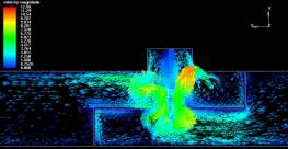
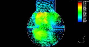
Figures 11-13 show the velocity profiles at 0, 650 (148 m3/hr), and 1100 GPM
(148 m3/hr) flow and 1750 RPM. ACUSOLVE puts a velocity vector at each node
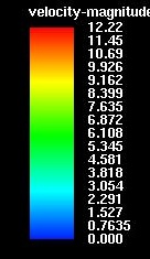
point of the mesh. The length of the vector and its color are based on the
velocity at that point. Bright red is always the highest velocity and typically
is seen at the tip of the impeller blades (tip speed). Dark blue is always zero.
All the other colors are in between. The values for yellow are given in Figures
10-12. Because the density of the mesh is highest near solid surfaces, it is
easily possible to get the impression that the intensity of mixing is highest
near the moving and stationary surfaces. It is not necessarily so. It is
important to look at the color and the length of the arrows before coming to
this conclusion. Because of the limitation of space, all figures in this paper
are available in a much larger size for viewing and analyzing at http://www.postmixing.com/
mixing%20forum/cfd_cfm/cfd_&_cfm.htm.
A vertical plane just behind the central plane is shown in Figures 11-13 to
eliminate the shaft and blades from view. Because the velocity is highest at the
tip of a blade, the large red arrows often mask out other more important
velocities. You can see them in some of the Axial shots, because the blades to
the right are coming toward you and are intersecting the plane of view.
| 0 GPM |
Radial Process Intensifier |
Axial Process Intensifier |
| Lightnin |
 |
 |
| |
Yellow = 8.7 m/s |
Yellow = 6.5 m/s |
| Hayward Gordon |
 |
 |
| |
Yellow = 9.3 m/s |
Yellow = 9.3 m/s |
|
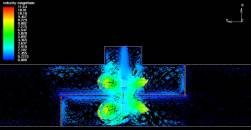
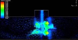
Figure 11: Velocity vectors at Q = 0 GPM, N = 1750 RPM.
This vertical plane was taken just behind the shaft. The mean
velocity entering the mixing zone is 0 m/s. |
Figure 11 shows the velocity vectors without any pipe flow. The flow pattern
can be inferred by connecting the arrows. Even though the impellers are working
very hard in this confined space, there are still several areas that appear to
be without big vectors. Both Axial units have almost no velocities in the
T-section of the pipe. Both of the upper impellers are down-pumpers. The radial
units are doing a better job in the T. The velocity vectors of the LTR do not
reach out to the ends of the Z-plate like the HGR does. The LTR will have
significant recirculation zones in the upper and lower chambers.
| 650 GPM |
Radial Process Intensifier |
Axial Process Intensifier |
| Lightnin |
 |
 |
| |
Yellow = 8.7 m/s |
Yellow = 6.5 m/s |
| Hayward Gordon |
 |
 |
| |
Yellow = 9.3 m/s |
Yellow = 9.3 m/s |
|
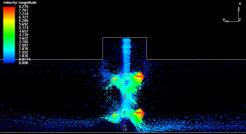
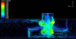
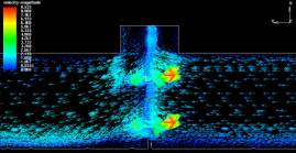
Figure 12: Velocity vectors at Q = 650 GPM, N = 1750 RPM.
This vertical plane was taken just behind the shaft. The mean
velocity entering the mixing zone is 0.81 m/s. See some interesting
animations at this
flow rate. Caution: These are very large files and the download
time is long, but well worth the wait. |
| 1100 GPM |
Radial Process Intensifier |
Axial Process Intensifier |
| Lightnin |
 |
 |
| |
Yellow = 8.7 m/s |
Yellow = 6.5 m/s |
| Hayward Gordon |
 |
 |
| |
Yellow = 9.3 m/s |
Yellow = 9.3 m/s |
|
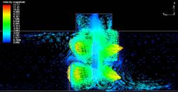
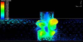
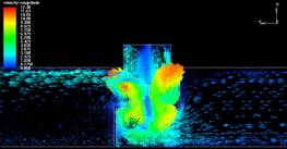
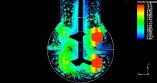
Figure 13: Velocity vectors at Q = 1100 GPM, N = 1750 RPM.
This vertical plane was taken just ibehind the shaft. The mean
velocity entering the mixing zone is 1.37 m/s. |
It is interesting to see how the flow patterns are different depending upon
the flow rate through the pipe. For 0 GPM, the flow can even be seen going to
the right. It is clear that HGR has a more optimized placement of the Z-plate
ends. Large recirculation zones result in the design of the LTR in the upper and
lower chambers. These are evident at all flow rates. Although the impeller style
is the same, the wider blades of HGR are obviously creating much more flow than
the LTR. The T-section of the pipe appears to be most active with the HGR (Fig.
11-14). It appears that a simple change could make this even more active (Part
2).
 |
 |
 |
| HGR just before the shaft |
HGR at the shaft |
 |
|
 |
| HGR just after the shaft |
HGR downstream from the active mixing zone |
|
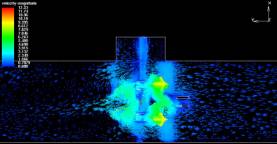
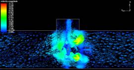
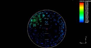
Figure 14: Pipe cross-sectional views of the HGR at 650 GPM and
1750 RPM. See the entire sequence of velocity vectors as an
animation from the beginning to the end of
the pipe. Caution: These are very large files and the download
time is long, but well worth the wait. |
The perspective of Figure 14 shows that there is a lot of swirl in the
Process Intensifier. Swirl is not conducive for mixing. Baffles are put in
vertical cylindrical tanks to stop the swirl. It looks as thought the Process
Intensifiers could use some sort of baffling, too. The two pictures on the left
in Fig. 14 show how strong the swirl is near the impellers and in the upper
T-section. This cannot be seen in Figures 11-13 because of the orientation. In
the top left picture of Fig. 14, the bottom half is the flow from the pipe
approaching the lower impeller. The top half is between the impeller and a
Z-plate end in the upper chamber. In the bottom left picture of Fig. 14, the
bottom half is the flow between the impeller and a Z-plate end in the lower
chamber. The top half is on the way out to the pipe. The picture on the top
right is taken directly through the shaft. The impellers are radial paddles. The
reason it does not look that way is because of the arrows drawn in over the
blades. The bottom right picture is in the pipe half way to the end. There is
noticeable clockwise swirl. The flow in the top left is coming back toward the
viewer. There are some very interesting dynamics in the outlet of these Process
Intensifiers. The larger scale is the same for all of these pictures.
It appears that the impeller diameter for LTA should be larger for these pipe
flow rates (Figures 12-13). At 0 GPM (Fig. 11) the flow from the upper impeller
appears to be reaching the bottom impeller slightly. For a better top-to-bottom
flow pattern, the impellers should be closer together. Perhaps 3 impellers of
this diameter would have been better. The spacing is 5 inches (127 mm) (or
S/D=1.43). Hydrofoils may have done a better job. It is obvious that as the pipe
flow rate is increased to 650 and 1100 GPM (148 and 250 m3/hr), the flow
patterns are completely staged. Flow from the center of the pipe appears to be
just sailing by the impellers with little interference (this will be more
evident when we look at tracers). The flow in the T appears to be almost
stagnant. It would appear that having more and larger impellers would help to
get a good top-to-bottom flow pattern and thus interrupt the general pipe flow
pattern. If the direction of the impellers were reversed, the T-section would
also be activated. This would minimize fluid elements from bypassing the active
mixing zone or getting stuck in this recirculation zone. More about this will be
presented in Part 2.
The up-pumping down-pumping combination of the HGA seems to keep the pipe
cross-section very active. The impinging zone between the impellers can be well
seen for 0 and 650 GPM (0 and 148 m3/hr). There is an asymmetry to this flow
pattern for 1100 GPM (250 m3/hr) directly after the flow straighteners in the
overall general flow direction. These flow straighteners may actually help the
pipe flow overwhelm the impeller flow pattern in this region. The volume in the
T-section also does not appear to be that active. It may be a source for
bypassing and recirculation. Recirculation zones create the long tail on
residence time distributions. This common occurrence in both LTA and HGA has to
do with the upper down-pumping impeller.
Continue with Flow Patterns
or Go back to Results
or Go
back to the Title Page
|